q0: Primitives for Hyper-Epoch Pretraining
Multi-epoch training is becoming the standard now that compute is growing faster than the supply of high-quality text. But pretraining a single model saturates within a few passes, long before the compute budget is exhausted. We argue this calls for a conceptual shift from training a single model toward exploring a population of models and aggregating their predictions.
The framing comes from Solomonoff induction [1], which says to keep many hypotheses for the data and weight them by a prior instead of betting everything on one. We do two things here. The first is the methodology. q0 turns a multi-epoch budget into a population through three primitives. A cyclic schedule collects diverse models quickly, chain distillation compounds their quality, and a learned prior weights them for any inference budget. The second is allocation. Building on our methodology, we work out how best to spend a given epoch budget, which shifts with its size, across the whole range from a single epoch up to the largest.
Primitive 1. Fast Exploration of Weight Space via Snapshot Ensembling
The obvious way to build a population is to train several models independently, each from its own random seed. But every run starts from scratch with no memory of what the others found, so you pay the full training cost again for each model.
Snapshot ensembling [2] gets the population of models from a single run, with no wasted restarts. The trick is a cyclic schedule. Training is divided into short cycles, and at each cycle end the learning rate has decayed to its floor while weight decay is at its peak, so the model has settled hard into a basin. Save that as a snapshot. Then the LR resets, giving the model enough energy to escape and settle somewhere new.
Primitive 2. Model Capability Compounding via Chain Distillation
loss low
loss
Snapshot ensembling gives you a population, but every member has still only seen one-hot labels. How good any single snapshot can get is capped by what cross-entropy can pull out of those labels, so a larger ensemble is mostly just more members of roughly the same quality. Chain distillation lifts that per-snapshot quality directly, by training on a richer signal than the labels alone.
After a few warmup cycles, each new snapshot trains against the one just before it, used as a frozen teacher and refreshed at every cycle boundary. Its loss keeps the usual next-token cross-entropy but adds a temperature-scaled KL term that pulls its predictions toward the teacher's:
$\mathcal{L}_{\text{CE}}$ is cross-entropy against the true next token
$z,\ z'$ are the student's logits and the frozen teacher's (the previous snapshot)
$\alpha$ sets how much to lean on the teacher versus the ground truth
$T$ is the softmax temperature, with $T^2$ keeping the KL gradient on the CE term's scale
The teacher's soft distribution carries more than a one-hot label does. Its probabilities on the wrong tokens reveal which ones it treats as similar, the dark knowledge that distillation [3] relies on, and its confidence on the correct token reweights how much each example contributes. In the spirit of born-again networks [4], where a model is retrained against an earlier copy, both effects make the supervision strictly richer than the labels.
Because each model conditions on its predecessor and improves on it, the population's capability compounds along the chain rather than flattening into members of similar quality. This does cost some diversity, since consecutive snapshots end up more alike. But the per-model quality gain outweighs that loss, and the diversity a single chain gives up is recovered by running several trajectories rather than one.
Primitive 3. Learned Generalization Prior
The first two primitives give us a pool of models, trained quickly and each better than a plain snapshot. Standard ensembling simply averages all of them with equal weight. But not every model helps the ensemble the same amount, and if your inference budget only lets you run $K$ of the pool, you have to choose which $K$.
The naive choice is the $K$ with the lowest individual loss. But the individually-best models aren't always the best ensemble. A slightly worse model can still correct mistakes the others share, so instead of ranking by individual loss, we learn which members to keep and how to weight them, fitting weights on a small held-out set that minimize the ensemble's loss:
$\mathcal{F}$ is a held-out fitness set the weights are fit on
$p_{i,t}$ is the probability member $i$ assigns to the true token at position $t$
$w$ are the mixture weights, a softmax over learned logits $\beta$
Because the weights mix the probabilities inside the log, they favor models that complement each other rather than the ones that merely look best on their own. The same fit is reused at any inference budget $K$.
How to allocate the budget
Chain distillation makes each model individually better, but it has a side effect. The models start to agree more, which removes some of the diversity between them. That matters, because an ensemble only helps when its members are both good and disagree.
We get the diversity back by running a few separate trajectories (base models) instead of one, each from a different random initialization. A base model is one run of the cyclic schedule with chain distillation, producing its own chain of snapshots. And it stays cheap. Rather than train many models from scratch to get diversity, we only run a few trajectories, and each one gives us many snapshots.
But you can't just run many tiny trajectories either. Given a fixed budget of total training epochs $E$, do you spend it all on one long trajectory, or split it across several shorter ones? Neither extreme wins. Every fresh trajectory pays a warm-up cost before its snapshots are any good, so splitting a small budget across many bases wastes most of it warming up. A single trajectory stretched too long does the opposite, with its late cycles drifting away from good minima. The sweet spot moves with the budget.
The optimal number of bases climbs in a rough staircase. One base wins up to around 128 epochs, two through about 256, three through about 512, and only past that does a fourth or fifth start to help. The gains flatten out after about three. Roughly speaking, each additional base wants a doubling of the epoch budget, so in most cases more cycles per trajectory is a better use of compute than more trajectories.
The small-budget regime
The plot above runs out to very large budgets, which may become routine as compute keeps growing. For now, though, the practical case is the other end, with only a handful of epochs to spend. From the allocation, these small budgets are best spent on a single base, since one trajectory beats splitting when epochs are scarce. But a handful of epochs is too little to spread the usual cyclic schedule across the whole run. So we keep the single trajectory and pack the cycles into the very end instead. We train normally for most of the budget, then run a short burst of cyclic LR cycles back-to-back, one snapshot per cycle.
We found that at a single epoch, four short cycles squeezed into the final fraction of training beat keeping one checkpoint. At four epochs, training three normally and then running the four short cycles through the last one does better still. The crossover we see lands around eight epochs. Below it, packing the cycles at the end wins. Above it, full cycles spread across the budget pay off and the staircase kicks in.
Results
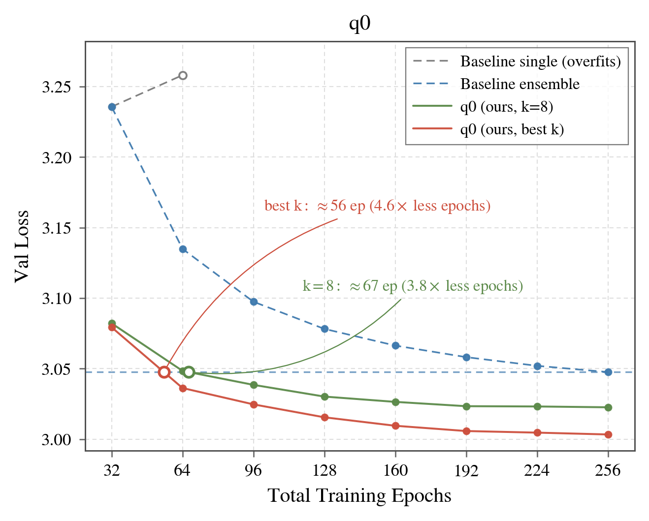
Everything above runs on a 1.8B-parameter decoder-only transformer trained on 100M FineWeb [5] tokens, with a disjoint 10M-token validation set. This is the fixed-data, infinite-compute setting of the Slowrun challenge [6], where the goal is to get the best performance out of a limited dataset. The baseline is a strong one, with eight models trained independently for 32 epochs each (256 in total) and their EMA weights averaged uniformly in probability space.
| method | epochs | val loss |
|---|---|---|
| baseline (naive ensemble) | 256 | 3.0476 |
| q0 | 256 | 3.0034 |
| q0 (scaled) | 960 | 2.9870 |
q0 reaches the 256-epoch baseline's loss at around 56 epochs, about 4.6× fewer epochs, or roughly 3.8× fewer when matched to the baseline's ensemble size of eight, and it continues to improve past it. Under the Slowrun data-efficiency accounting, that comes to a data efficiency of about 12.9×.
The gains aren't confined to validation loss. They transfer to zero-shot downstream benchmarks, where q0 improves over the baseline on every task, and we find a data efficiency of about 14.2× (16.0× for the scaled run) against 12.2× for the baseline:
| method | ARC-E | PIQA | SciQ | avg |
|---|---|---|---|---|
| baseline | 0.4781 | 0.6697 | 0.7850 | 0.6443 |
| q0 | 0.4865 | 0.6823 | 0.8030 | 0.6573 |
| q0 (scaled) | 0.4945 | 0.6774 | 0.8080 | 0.6600 |
We hope q0 encourages further work on multi-epoch pretraining as a way of scaling compute over limited data, especially by efficiently searching for diverse models. Searching over a population is a different problem than training a single model with gradient descent, and likely calls for new primitives; the three we introduce here are a first set that give large gains, and we expect much more lies ahead.
Full paper on arXiv.
References
- R. J. Solomonoff. A formal theory of inductive inference. Information and Control 7(1), pp. 1–22, 1964.
- G. Huang, Y. Li, G. Pleiss, Z. Liu, J. E. Hopcroft, K. Q. Weinberger. Snapshot ensembles: train 1, get M for free. ICLR, 2017.
- G. Hinton, O. Vinyals, J. Dean. Distilling the knowledge in a neural network. 2015.
- T. Furlanello, Z. C. Lipton, M. Tschannen, L. Itti, A. Anandkumar. Born-again neural networks. ICML, 2018.
- G. Penedo, H. Kydlíček, L. Ben Allal, A. Lozhkov, M. Mitchell, C. Raffel, L. Von Werra, T. Wolf. The FineWeb datasets: decanting the web for the finest text data at scale. NeurIPS Datasets and Benchmarks, 2024.
- Slowrun: a benchmark for language modeling in the fixed-data, infinite-compute regime. github.com/qlabs-eng/slowrun.